MSc research · FAU Erlangen-Nürnberg

Six drones, one formation, no GPS.

Distributed moving-horizon estimation and model-predictive control for heterogeneous UAV clusters — quaternion hexacopters and 6-DOF fixed-wing aircraft, each agent running its own constrained real-time estimator and controller, coordinating over a communication graph with no central node.
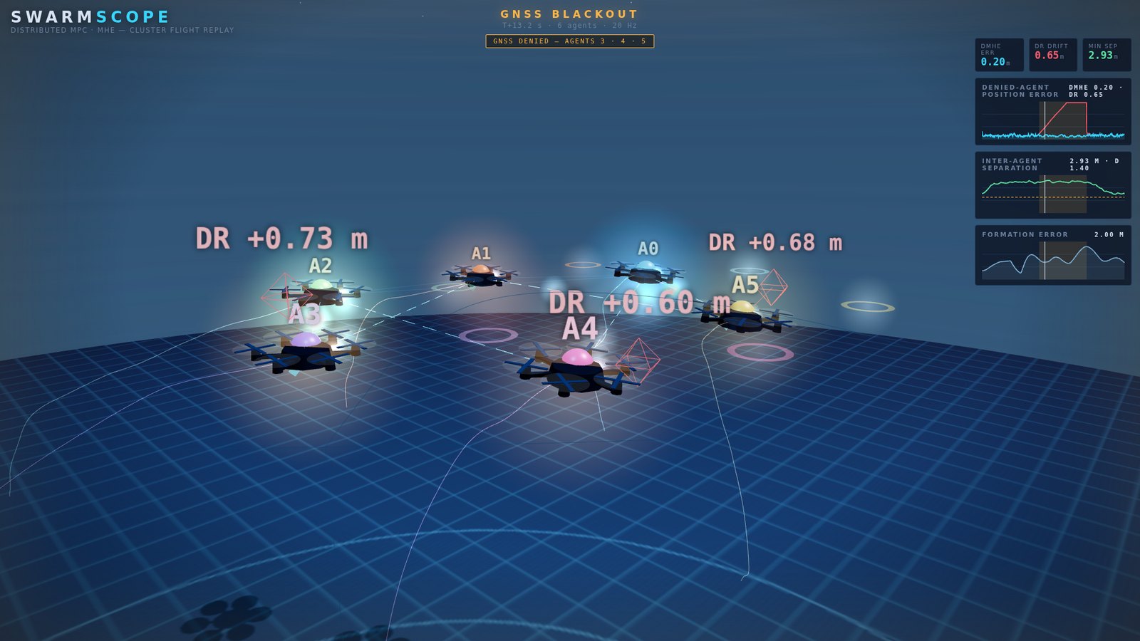
Six hexacopters in formation during a GNSS blackout; red wireframe markers show where dead reckoning believes three of them are, more than a metre from the truth. T+13.2 s — GNSS denied, agents 3·4·5. Red wireframes are the dead-reckoning estimate drifting away from the truth; the aircraft themselves stay on station. Click to fly the mission yourself.
Denied-agent error
0.088 m
through a 10 s GNSS blackout — against 1.26 m dead-reckoning
Monte-Carlo campaign
210 runs
0 divergences, 0 solver failures across every scenario
Min separation
1.55 m
against a 1.40 m barrier radius — 0 breaches nominally
Solvers in the loop
76 µs
per agent per cycle, compiled C estimator + controller
The problem

What happens when the map goes dark

A formation of drones is only as good as each agent's idea of where it is. Lose GNSS — under a bridge, in a canyon, indoors, jammed — and a dead-reckoning filter drifts within seconds. In a tight formation that drift is not merely an inaccuracy: it is a collision.

This project builds the distributed alternative. Every agent keeps its own moving-horizon estimator and its own predictive controller; agents exchange estimates and relative measurements with their graph neighbours, and nothing is centralised. When an agent loses its absolute fix, it fuses relative measurements to neighbours that still have one, and stays localised to centimetres while the formation keeps flying and keeps its separation.

The mission below is the one the replay shows, and it is the one every figure on this page comes from: six hexacopters take off, assemble a ring, translate as a body, and then contract and rotate the formation — while three of the six are GNSS-denied for ten seconds in the middle of it.

take-off · assembly sweep GNSS blackout · agents 3·4·5 contract + rotate 0 s8 1222 30
The 30-second reference mission. The blackout window deliberately overlaps the start of the reconfiguration, so the estimator is tested while the formation geometry is changing underneath it.
Architecture

The loop each agent closes

Estimation, control and safety are separate blocks with separate jobs, and the coupling to the rest of the cluster enters at exactly three points.

sensors GNSS · IMU · rel. DMHE moving-horizon estimator DMPC predictive controller CBF filter safety plant 13-state x̂ a_des u measured state · 20 Hz neighbours over the communication graph estimates + covariances · slot consensus relative meas. slot ref. neighbour pos.
One agent, one sample. The estimator fuses its own sensors with neighbour information; the controller tracks a formation slot agreed by consensus; the barrier filter is the last thing the command passes before the plant, so separation is enforced on the input that is actually applied, not on the one that was planned. Everything shown here runs on every agent, at 20 Hz, with no central node.
Software

Three layers, one interface

The numerical core is C, the coordination logic is C++, and the research layer — models, missions, campaigns, figures — is Python. The layers meet at a small allocation-free C interface: set the reference, push constraint rows, prepare, feed back.

That boundary is load-bearing rather than decorative. The coordination layer never sees how a solver is built, so the repository ships a dependency-free reference implementation behind the same interface and the whole stack runs standalone.

Python — models · missions · campaigns hexacopter · fixedwing · mc_study C++ — coordination layer DMHE fusion · consensus · CBF filter C interface — uav_solver.h set_reference · set_constraint_bounds · prepare · feedback reference core LQR + information filter ships in this repo real-time solver RTI NMPC + MHE separate work either core — nothing above changes
The two cores are interchangeable from the layer above. Every distributed result on this page was produced with the reference core, and reproduced with the compiled real-time core substituted in.
Vehicle models

Two airframes, derived from first principles

Both models are derived in the report from Newton–Euler mechanics with every frame, relation and Jacobian stated explicitly — and both are checked numerically before any control result is claimed.

13 states · quaternion attitude

Hexacopter

Attitude is carried as a unit quaternion rather than Euler angles, so the model has no gimbal singularity anywhere in the flight envelope:

q̇ = ½ · q ⊗ [0, ω] ‖q‖ = 1 preserved exactly

Six rotors drive a four-dimensional wrench, so allocation is over-actuated: the mixer M ∈ ℝ4×6 has rank 4 and a two-dimensional null space, which is what gives the airframe its single-rotor-failure margin. Thrust and reaction torque follow the standard kfΩ² / kmΩ² laws with alternating spin directions.

Control runs as differential flatness into a geometric SO(3) attitude loop, so the predictive layer plans in position while attitude tracking stays on the manifold.

6-DOF · Beard–McLain · Aerosonde

Fixed-wing

The full rigid-body aerodynamic model: wind triangle, sigmoid-blended stall aerodynamics so lift is valid past the linear region, complete force and moment coefficient expansions, and product-of-inertia rotational dynamics in Γ form.

CL(α) = (1−σ)·CL0+CLαα + σ·2·sign(α)sin²α cos α

Straight-and-level trim is solved numerically rather than assumed — at Va = 35 m/s it lands at α = 0.20°, δe = −2.83°, δt = 0.464 — and a cascaded autopilot with look-ahead guidance flies the coordinated-turn echelon loiter.

Four aircraft hold the loiter at 120 m with 35.5 m mean spacing; ten different initial-condition seeds converge to the same limit cycle.

Validated, not asserted. validate_models.py checks quaternion group properties and the exponential map, mixer rank and allocation round-trips, hover equilibrium, rigid-body energy consistency, the wind triangle, stall blending and the computed trim — and prints ALL CHECKS PASSED. Everything downstream rests on that.
Distributed estimation

Anchor coverage

The campaign was built to find where distributed estimation breaks. It does not degrade smoothly with how many agents lose GNSS — it falls off a cliff, and the cliff is a property of the communication graph.

A GNSS-denied agent can stay localised only if it can see someone who is not lost. Fusing a relative measurement to a neighbour transfers that neighbour's confidence — weighted by its covariance, so a shaky anchor contributes little — but a ring of agents who have all lost their fix has nothing to transfer between them, and the whole cluster drifts together.

COVERED — 3 OF 6 DENIED 012 345 error 0.091 m · sep 1.55 m BROKEN — RING, 5 OF 6 DENIED 012 345 error 0.506 m · sep 0.98 m · breaches MULTI-HOP — LEVELLED DAG 012 345 ℓ0 ℓ1 ℓ2 ℓ3 ℓ2 ℓ1 error 0.111 m · sep 1.49 m · 0 breaches
Green holds GNSS · amber is denied but anchored · red is denied with nothing to anchor to. Cyan arrows are relative-measurement fusion, pointing at the agent whose confidence is being borrowed; faint lines are the communication graph. Left, the nominal mission — each denied agent borders a localised neighbour, over the ring or a two-hop chord. Middle, the failure the sweep exposed: on a plain ring with five of six denied, only the survivor's two ring neighbours can anchor at all, and the three agents beyond them drift as a body until separation is breached. Right, the repair: each agent takes an anchor level — the survivor is ℓ0, its neighbours ℓ1, theirs ℓ2 — and may fuse only toward a strictly lower level. That makes the anchor relation a DAG, so the fix propagates outward hop by hop and no agent ever re-absorbs its own estimate through a loop.

Why covariance-weighting matters

A relative measurement y = pi − pj is only as good as the neighbour's own position. Fusing it as though p̂j were truth injects the neighbour's error straight into your estimate; the rule used here inflates the measurement covariance by the neighbour's reported covariance, Rrel + Pj, so an anchor that is itself uncertain is discounted automatically.

Two further rules keep the fusion honest: it triggers only on loss of the absolute fix, so a healthy agent never degrades itself with stale neighbour information, and it runs in two passes per sample, so every agent anchors to same-step estimates rather than to yesterday's.

What the estimator actually is

Each agent runs a constrained moving-horizon estimator over a window of past measurements, with an arrival cost carrying everything older than the window. On the linear translational sub-problem it reduces exactly to an information-form Kalman filter, which is what the reference implementation here uses — a property the report derives rather than assumes.

That reduction is the reason the distributed layer can be studied honestly with the reference core: the coupling, the anchoring policy and the covariance arithmetic are identical whichever core sits underneath.

Results

210 runs, zero divergences

Single missions prove nothing. The claims below come from a Monte-Carlo campaign over noise realisations, denial severities, degraded graphs, estimator ablations and solver substitutions — all reproducible from mc_results.json in the repository.

Blackout: estimate vs. dead reckoning

Mean position error of the three denied agents, reference mission (seed 7)
DMHE dead reckoning GNSS denied

Denial sweep & the coverage cliff

Denied-agent RMSE against number of agents denied, 12 seeds each
DMHE, one-hop multi-hop anchoring p95

Compiled solvers in the closed loop

15 paired seeds per configuration — identical noise streams
denied-agent RMSE [m] min separation [m]

Per-agent solver cycle

Preparation time, single core, median of best-of-seven
rebuilt each sample warm-started
The estimator earns its place. Ablating it — flying the same missions with a per-agent filter and no relative fusion — leaves estimation looking deceptively fine (0.089 m, because the non-denied agents dominate the average) while formation keeping degrades by 4.8× and minimum separation falls to 0.75 m, well inside the 1.40 m barrier. The failure appears in the geometry, not in the error statistic.

Every scenario

ScenariorunsRMSE meanmedianp95 shape errmin sepbreachesdiv.
Nominal — 3 of 6 denied300.0910.0910.0990.0941.5500
1 of 6 denied120.0680.0680.0740.1031.4900
2 of 6 denied120.0780.0780.0850.0951.5400
4 of 6 denied120.1060.1050.1170.0871.5400
5 of 6 — coverage broken120.4510.3650.6890.2180.90yes0
5 of 6 — multi-hop120.1190.1200.1270.0681.4900
Ring graph — coverage broken120.5060.4740.7990.2310.98yes0
Ring graph — multi-hop120.1110.1120.1190.0981.4900
Communication edge dropped120.0940.0920.1070.0951.5000
Distributed estimator ablated120.0890.0870.0990.4200.75yes0
Reference core in the loop150.0910.0900.1000.0931.5500
Compiled estimator + controller150.0620.0620.0700.0961.5300

Errors in metres. “Shape error” is formation geometry error with the cluster centroid removed; “breaches” counts samples below the 1.40 m barrier radius. Divergence and solver-failure counts are zero in every row of the campaign.

Interactive

SwarmScope

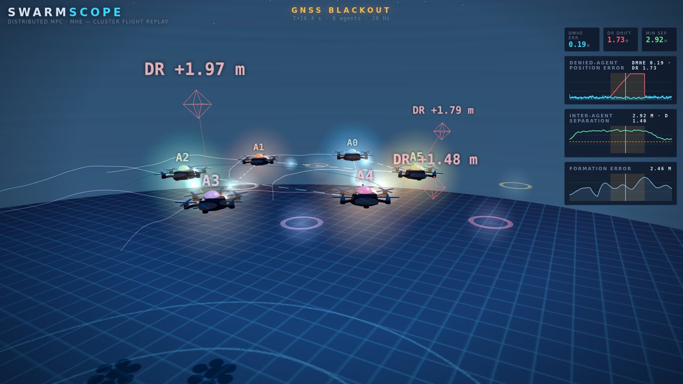
The same mission, in 3D, replayed from the logged data — not an animation of it.

Every position, attitude quaternion, estimate and metric in the replay is read straight from the simulation output. Watch the blackout hit at T+12 s, the dead-reckoning ghosts peel away from the aircraft, the fusion beams light up to GNSS-good neighbours, and the formation contract and rotate with the closest-pair separation called out against the barrier radius.

  • Cinematic, orbit, top-down and per-agent chase cameras
  • Live telemetry charts with a scrubbable mission timeline
  • A second scene: the four-aircraft fixed-wing echelon loiter
SwarmScope replay showing six hexacopters in formation with telemetry panels and a mission scrubber.
The code

Run it yourself

Clone, install NumPy, and every result on this page reproduces on your machine.

# clone and validate the models
git clone https://github.com/anilram30/uav-cluster-dmpc-dmhe
cd uav-cluster-dmpc-dmhe/python
pip install -r requirements.txt

python3 validate_models.py   # -> ALL CHECKS PASSED
python3 sim_hexacluster.py   # the reference mission
python3 sim_fixedwing.py     # echelon loiter
python3 make_figures.py      # regenerate figures/
# the scenarios behind the results table
from sim_hexacluster import run

run(denied=(1,2,3,4,5), topology='ring')
run(denied=(1,2,3,4,5), topology='ring', multihop=True)
run(ctrl_est='ekf')        # ablate the estimator
run(edge_drop=(0,1))      # degrade the graph
c_api/ C numerical core uav_solver.h the interface — MPC + MHE uav_solver_ref.c reference implementation cpp/ C++ coordination layer agent.hpp fusion · consensus · CBF cluster_demo.cpp end-to-end smoke test python/ research layer uavdmpc/ models, control, estimation sim_hexacluster.py sim_fixedwing.py mc_study.py 126-run campaign mc_study2.py 84-run campaign make_figures.py figures/ generated figures docs/ this site + SwarmScope report/ technical report (PDF)
On the solvers. The per-agent real-time-iteration NMPC controller and MHE estimator used for the in-the-loop and timing results are my own separate research work — an extension of my MSc thesis on SLQP-MPC, with the estimator being the moving-horizon counterpart of the same solver. That work is ongoing and not yet published, so its algorithms and sources are not part of this repository, and the report here is a public edition that specifies the solvers by the problems they solve, the real-time pattern they run in, the interface they are reached through and their measured timing. The distributed framework depends on none of it: the reference implementations shipped here satisfy the same interface, and everything reproduces standalone.